GAUSS helps you to solve numeric optimisation problems and is often used in statistics, econometrics and time series analysis. It is often used in economics, portfolio-management or in technical applications, as well. No other product offers the same combination of interactive tools for data analysis, precision in calculations and speed and efficiency!
Based on a matrix-oriented programming language GAUSS is the number one product wherever innovative and computer-intensive problems occur. GAUSS is optimized for rapid prototyping and the application of numerical algorithms for data analysis. Desktop and enterprise edition are equipped with a 64-bit-compiler that allows scalable implementation of numerical methods.
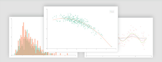
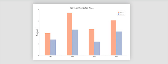
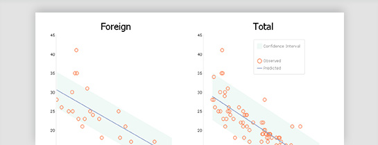
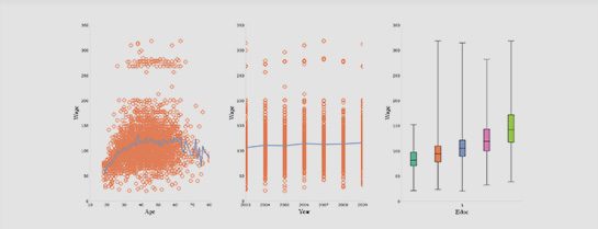
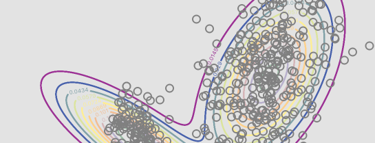
At the same time GAUSS offers an interactive data evaluation suite that does not require much programming skills from the user. It can easily produce high-professional graphs like 2D- and 3D-plots, surface- and Box-plots or histograms.
Its flexibility makes GAUSS the first choice for statisticians, economic and financial analysts.
Arguments for GAUSS:
- Easy to learn and fast programming language
- More than 400 predefined mathematical functions
- Allows data analysis for big data
Gauss - Mathematical and Statistical System
The GAUSS Mathematical and Statistical System is a fast matrix programming language widely used by scientists, engineers, statisticians, biometricians, econometricians, and financial analysts. Designed for computationally intensive tasks, the GAUSS system is ideally suited for the researcher who does not have the time required to develop programs in C or FORTRAN but finds that most statistical or mathematical "packages" are not flexible or powerful enough to perform complicated analysis or to work on large problems.
Whatever mathematical tool or language you are now using, you'll find that GAUSS can greatly increase your productivity!
Comprehensive Environment for Modeling and Analysis
GAUSS is a complete analysis environment suitable for performing quick calculations, complex analysis of millions of data points, or anything in between. Whether you are new to computerized analysis or a seasoned programmer, the GAUSS family of products combine to offer you an easy to learn environment that is powerful and versatile enough for virtually any numerical task. Since its introduction in 1984, GAUSS has been a standard for serious number crunching and complex modeling of large-scale data.
Worldwide acceptance and use in government, industry and the academic community is a firm testament to its power and versatility. The GAUSS System can be described several ways: It is an exceptionally efficient number cruncher, a comprehensive programming language, and an interactive analysis environment. GAUSS may be the only numerical tool you will ever need.
Interactive and Fast
For simple problems GAUSS provides a fully interactive environment for exploring data, creating scenarios and analyzing results. For more complex tasks, you can write programs and save them to disk. GAUSS is exceptionally fast, providing performance comparable to compiled C or FORTRAN programs. And unlike other math packages, GAUSS's speed is equally impressive when working with problems of very large scale.
Straightforward and Efficient
While many GAUSS users never find a need to program extensively, for those who do, GAUSS provides a natural and logical environment that is easy to learn and powerful to use. At the core of GAUSS is an efficient programming language adequate for doing even the most sophisticated analysis. The basic unit of analysis in GAUSS is a matrix, resulting in a syntax closely resembling common mathematical expressions. Since matrix operations are assumed, most of the looping required by other languages is eliminated.
The Data Translation Loop allows transformations on variables in a data set by directly using the variable names in expressions. This streamlines data transformations and makes for shorter, more readable programs. GAUSS's Source Level Debugger greatly simplifies program development. With all of the features you would expect in a dedicated debugging system, you can quickly identify and solve program logic errors at run time.
Additionally, GAUSS handles complex numbers automatically and seamlessly. You don't have to keep track of the real and imaginary parts of a matrix. Complex numbers are handled automatically, that greatly simplifies programming for engineering and other tasks that require working with complex numbers.
The Language
As a complete programming language, the GAUSS system is both flexible and powerful. Immediately available to the GAUSS user is a wide variety of statistical, mathematical and matrix handling routines.
GAUSS can be used either interactively for short one-off commands or by creating large programs consisting of several files and libraries of functions, or anything in between.
Visualization and Presentation
GAUSS's high resolution Publication Quality Graphics gives you powerful ways to visually analyze your data and present your findings. A wide choice of graphing options are available to you, including 2D, 3D, surface, contour, polar and log graphs, as well as bar graphs, histograms, box graphs and more. Graphs can be placed in individual overlapping or tiled windows on a single page. You can export graphics files in a number of popular formats, including WMF, HP-GL/2, PostScript and EPS formats, for use in page layout and presentation packages, and GAUSS includes support for a wide range of output devices, including most of the latest printers and plotters.
The Tools You Need
GAUSS has over 400 mathematical functions built in, including LINPACK, EISPACK and BLAS routines, factorizations, decompositions, eigenvalues, distributions and equation solving functions, to provide you with all the tools you need to solve your most difficult problems. You can easily customize or add to the GAUSS function library, and optional modules provide access to many other specialized capabilities.
The GAUSS Run-Time Module (GRTM) allows users to distribute GAUSS applications that they have written to people who do not have GAUSS. Developers distribute a compiled file to end users along with the GRTM. This is available with GAUSS at no extra charge.
Other important features include: data import/export compatibility with many popular spreadsheets and databases, long period random number generators, built-in functions for efficiently handling sparse data, and a Foreign Language Interface for incorporating your favorite compiled C and FORTRAN programs directly into GAUSS programs.
Further Information:
System Requirements
The GAUSS Data Tool 10 is available for Windows in the 32- and 64-bit variants. The Windows 32-bit version works on a 64-bit PC, but not the other way around. In addition, the 64-bit Windows version of the GDT 10 does not have a graphical user interface.
What's New in GAUSS
Expanded suite of date and time tools
- Easily convert dates between many formats.
- Generate date vectors of varying frequency and length.
- New functions to transform and operate on times and dates.
- New support for high-frequency data.
Quantile regression
- Perform conditional quantile regressions using interior-point or quadratic programming algorithms.
- Estimate local linear or quadratic regressions.
- Compute bootstrapped standard errors and confidence intervals.
New online license activation
Get started faster with seamless online license activation from a product key.
Faster fundamental computations
- Multiply arrays with 50 or more elements 20% to 3,500% faster.
- Invert matrices 20%-400% faster.
- Faster log, ln, and exp functions.
- Increased matrix multiplication speed for non-square matrices.
Expanded covariance computations
- New cluster-robust and heteroscedastic-robust covariance computations.
- Use as stand-alone functions or with OLS regressions.
- Compute outer product of gradients (OPG) covariance after optimization.
New graphics tools
- Plot high-frequency and irregular time series data.
- plotTS now supports daily data.
- Simple controls for tick label locations in 2-D graphs.
- New controls for box plot grouping.
Enhanced user interface
- New convenience features.
- Improved HiDPI support.
- Updated icons and flatter UI style.
Other new mathematical functions
- impute fills missing data with mean or median values (more options to come).
- norm matrix 1, 2 (Spectral), Infinity, Frobenius and Nuclear norms or the vector p-norm.
- lagTrim returns a matrix containing specified lags and/or leads with incomplete rows removed.
- recservar performs efficient simulation of a VAR model.
- saved now provides a simple way to save datasets in CSV, or XLS/XLSX
Move from data to results more efficiently than ever with GAUSS. GAUSS new features improve data reading and handling capabilities, expand built-in analytical and graphic tools and significantly increase computation speeds.
- Improved data handling
- General Method of Moments
- Graphics Functionality
- New Productivity Functions
- Speed Improvements
- Mathematical functions
Improved data handling
Load, transform and analyze in one line. Simple to use formula string notation supports:- NEW formula strings
- Read SAS and STATA datasets
- Improved Handling of Large Datasets
NEW formula strings simplify loading and transforming data
//Load data, transform and estimate in one step
call ols("credit.xlsx", "ln(balance) ~ ln(income) + factor(sex)");
//Load data, reclassifying string column 'state' into numerical categories
X = loadd("census.csv", "income + household_size + reclassify(state)");
GAUSS expands the previously integrated formula string syntax to allow single line data loading, transformation, and analysis. The enhanced formula string syntax :
- Drastically decreases required lines of code.
- Works with CSV, Excel, GAUSS datasets, HDF5, SAS and STATA datasets.
- Supported automated transformations include:
- apply transformations, such as `ln`, `exp` or any GAUSS procedure
- create interaction terms
- create dummy variables
- reclassify string variables
Read SAS and STATA datasets
//Load SAS dataset, create interaction term and assign to GAUSS matrix 'X'
X = loadd("advertising.7bdat", "sales + radio * billboards + direct_mail");
//Load Stata dataset and compute descriptive statistics
call dstatmt("auto2.dta", "mpg + weight + gear_ratio");
Sharing data between GAUSS and other software just got easier. Not only does GAUSS 18 allow you to read SAS and STATA datasets, it also allows you to use SAS and STATA datasets directly as a dataset for functions such as OLS, GLM and the General Method of Moments.
- Complete compatibility with SAS and STATA datasets.
- Import SAS and STATA datasets as data matrices.
- Use SAS and STATA datasets as direct arguments in functions such as OLS, GLM and the GMM.
Improved Handling of Large Datasets
//Load large data in consecutive 1 GB blocks
setBlockSize("1G");
//Load large data in consecutive blocks no larger than 10% of system memory
setBlockSize("10%");
GAUSS makes it easy to access and analyze large datasets with new, simple tools for controlling data processing. Users can now control data processing in terms of:
- Percentage of available memory.
- Simple memory specification.
- Number of rows.
More Features in GAUSS
The new Import Wizard
The new import wizard in GAUSS comes with a new fresh inituitive interface and now reads CSV, XLS, XLSX and other delimited text files. The import wizard is also able to handle malformed data files. Furthermore the speed of loading data and of the preview got improved. There is now a visual feedback and an enhanced experience with color coding.
Reclassification and Recoding
GAUSS provides new functions for an easy transformation of categorial variables from text labels to numeric labels and vice versa, or placing numeric ranges into seperated categories.
Reclassify
With this function you will be able to:
- reclassify text labels to numeric category labels
- reclassify numeric labels to text labels
- reclassify vectors individually, an entire matrix or a multidimensional array
//Create a 7x1 string vector X = "EU" $| "GBP" $| "USD" $| "GBP" $| "USD" $| "EU" $| "EU"; //Use 'uniquesa' to create a string vector //with the unique strings in 'X' listed //in alphabetical order from = uniquesa(X); //Create 3x1 vector of numeric category labels to = { 0, 1, 2 }; //Reclassify elements in 'X' from // EU -> 0 // GBP -> 1 // USD -> 2 X_numeric = reclassify(X, from, to);
Data Scaling - rescale Function
Maximum likelihood estimations or optimization routines often fail due to poorly scaled data. The new function rescale provides 8 different scaling options with one simple line of code.
Example: Use a named method and return the data plus scaling factors:
//Scale each column of 'x_train' { x_train, location, scale } = rescale(x_train, standardize");
In this example location and scale were passed in later to scale another sample from the same data set:
//Scale each column of 'x_test' with scale and
//location parameters created from training data above
x_test = rescale(x_test, location, scale);
Sample without replacement
//Take a 100 observation sample from 'x'
//without replacement
sample = sampleData(x, 100);
Sample with replacement
replace = 1;
//Take a 100 observation sample from 'x'
//WITH replacement
sample = sampleData(x, 100, replace);
Create training set and test set
n = rows(x); //Create indices for training set idx_train = sampleData(seqa(1,1,n), 0.75 * n); //Extract training set x_train = x[idx_train]; //Remove (or delete) training set rows from 'x' //to create test set x_test = delrows(x, idx_train);
Create random indices to draw from multiple variables
//Create random integers from between 1 and 1000 range = { 1, 1000 }; idx = rndi(50, 1, range); //Sample same observations from 'x' and 'y' x_sample = x[idx,.]; y_sample = y[idx];
Generalized Linear Model
In statistics, the generalized linear model (GLM) is a flexible generalization of ordinary linear regression that allows for response variables that have error distribution models other than a normal distribution. The GLM generalizes linear regression by allowing the linear model to be related to the response variable via a link function and by allowing the magnitude of the variance of each measurement to be a function of its predicted value. The GAUSS function glm is used to solve generalized linear model problems. GAUSS provides the following combinations from exponential family and related link function:
- Normal: identity, inverse, ln
- Binomial: identity, inverse, ln, logit, probit
- Poisson: identity, inverse, ln
- Gamma: identity, inverse, ln
Format
// Read data matrix from a '.csv' file and start from the second row data = csvReadM("binary.csv", 2); // Read headers from first row vnames = csvReadSA("binary.csv", 1|1); // Specify dependent variable y = data[.,1]; // Specify independent variable x = data[.,2:4]; // Specify link function link = "logit"; // Call glm function call glm(y, x, "binomial", vnames, 3, link);
Output
Generalized Linear Model Valid cases: 400 Dependent Variable: admit Degrees of freedom: 394 Distribution: binomial Deviance: 458.5 Link function: logit Pearson Chi-square: 397.5 AIC: 470.5 Log likelihood: -229.3 BIC: 494.5 Dispersion: 1 Iterations: 4 Standard Prob Variable Estimate Error z-value >|z| ---------------- ------------ ------------ ------------ ------------ CONSTANT -3.99 1.14 -3.5001 0.000465027 rank 2 -0.67544 0.31649 -2.1342 0.0328288 3 -1.3402 0.34531 -3.8812 0.000103942 4 -1.5515 0.41783 -3.7131 0.000204711 gre 0.0022644 0.001094 2.0699 0.0384651 gpa 0.80404 0.33182 2.4231 0.0153879 Note: Dispersion parameter for BINOMIAL distribution taken to be 1
Simplified Function Calls
Many GAUSS procedures used to require passing in all arguments including control structures. Additionally many GAUSS procedures that call a user-defined procedure, such as optimization or integration functions used to require extra data to be passed in as a DS structure. Now you just need the function integrate1d!
Old style
//Define procedure to be integrated proc (1) = myProc(x, struct DS d); local y; y = d.dataMatrix; retp(exp( -(x .* x) / (2 .* y) )); endp; //Define limits of integration x_min = -1000; x_max = 1000; //Define extra argument for procedure 'myProc' struct DS d; d = dsCreate(); d.datamatrix = 3; //Define 'ctl' to be a control structure struct integrateControl ctl; //Fill in with default values ctl = integrateControlCreate(); //Calculate integral integral = integrate1d(&myProc, x_min, x_max, d, ctl);
New simpler style
//Define procedure to be integrated proc (1) = myProc(x, z); retp(exp( -(x .* x) / (2 .* z) )); endp; //Define limits of integration x_min = -1000; x_max = 1000; //Define extra arguments for procedure 'myProc' a = 3; //No need for control structure if using default values integral = integrate1d(&myProc, x_min, x_max, a);
- QZ decomposition with options to sort the eigenvalues (qz)
- Hypergeometric CDF, PDF and random number generation (cdfHyperGeo, pdfHyperGeo, rndHyperGeo)
- Binomial PDF and Poisson PDF (pdfBinomial, pdfPoisson)
- Option to sort eigenvalues of generalized schur decomposition (qz)
- More powerful and easy to use integration function, using adaptive quadrature (integrate1d)
- Function to set axes line color and thickness (plotSetAxesPen)
- Option to specify range of random integers created by rndi
- Option to specify delimiter for strsplit
- Data sampling function, sampleData
- Data scaling function, rescale
- New functions for reclassifying data based upon a match (string or numeric) or a range, (reclassify, reclassifyCuts)
- Generalized Linear Model (GLM)
- Much improved, faster and simpler to use functions for reading CSV and other delimited text files (csvReadM, csvReadSA)
User Interface and other Enhancements
- Syntax highlighting and brace-matching in program input/output window
- Debugger page supports file editing, 'find usages' and full editor functionality
- Improved file associations on Mac
- Bug fixes