Dose response curves
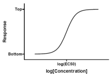
Dose-response sigmoid function (Sigmoidal Dose-Response).
Equitation: Y = Bottom + (Top − Bottom) / 1 + 10 log( EC 50) − X
Parameter: Top – maximum effect
Bottom – Effect at dosage 0 (resp. <<)
log EC 501 / 2 – Logarithm of the EC50 (turning point)
General, Agonist, Antagonist
Dose-response curves can be used as models for many different experiments. Typically, X denotes the concentration of the drug or hormone and Y denotes the biological response variable under investigation, e.g., enzyme activity, membrane potential, or contraction of a muscle. The term "dose" is interpreted relatively broadly, not only in the narrow sense of a drug administered to a human or animal at various concentrations. Likewise, it is used for in vitro experiments, and occasionally even for X variables such as temperature or voltage. An agonist is a substance that binds to a receptor and causes a response. If this response is stimulation as a function of dosage, the dose-response curve will be uphill from a low level at small concentrations to a high level at higher concentrations. If the agonist causes an inhibitory response, the dose-response curve will run inversely from a high level to a low level for high concentrations. An antagonist does not cause a response itself, but blocks an agonist-driven response. Therefore, if one varies the concentration of an antagonist (while keeping the concentration of an associated agonist constant), the dose-response curve will describe exactly the reverse of the associated curve of the agonist. The above function generally describes a relationship between a concentration of a substance or enzyme and the associated response, e.g., an effect. It is also called a logistic function with 3 parameters. This runs in an S-shape from a low level (bottom) to a high level of maximum effect (top).
Why a logarithmic X-scale?
A logarithmic X-scale is common because the agonist concentration typically spans several orders of magnitude. Therefore, graphical representation using a logarithmic scale is considerably easier. The concentration is often increased by a constant factor. This results in equidistant points on the logarithmic scale. Finally, the error of the EC50estimator is not normally distributed on a linear scale, a requirement for many analyses. If X is scaled linearly rather than logarithmically, the response curve is just a simple binding function (one-site binding) as in 3.1. EC50, ED50, IC50 For S-shaped curves, there is exactly one X-value at which the mean level between bottom and top is reached. This point is called EC50 ("effective concentration 50%") or ED50 ("effective dose 50%") or IC50 ("inhibitory concentration 50%") in case of a falling curve. In the formulas, the symbol logEC50 is used to remind that the X-axis is scaled logarithmically. By definition, EC50 depends on the bottom and top levels. It is one of 4 parameters that define the location of the dose-response curve. Therefore, the EC50 is often used as a measure of the potency of an agonist. Note, however, that the EC50 is not directly related to the dissociation constant K d , so it is not a direct measure of the affinity of the ligand-receptor pair. An alternative measure of agonist strength is the pEC50, the negative 10 logarithm of the EC50. pEC 50 := -log( EC 50) Often, the pEC50 is more convenient to handle because the EC50 is measured in nanromoles or micromoles. For example, if EC50 = 167 nM, pEC50 = 6.78
Gradient - constant or variable?
In this dose-response curve, the slope behavior is fixed. It is characteristic that for the increase from 10% above Bottom to 90% not quite two logarithmic units on the X-axis (more precisely: factor 81) are required. If this requirement is not met, an additional parameter must be introduced into the model.