Non-constant variance in the residuals of a regression analysis need not always be a problem. Although the least squares method assumes homoskedasticity (=constant variance), there are more flexible methods that do without this assumption. Loglinear Variance Models do not only allow correct significance statements in the presence of heteroskedasticity. With this class of models, presented here, one can simultaneously learn something about the technical causes of increased dispersion. 

Introduction and example 

Let's take a look at the following data:

A partial factorial test design is available, which was carried out by the National Railway Corporation of Japan [described in: G.Smyth 2002, original: Taguchi & Wu 1980]. This was used to investigate the influence of nine factors on the tensile strength of welds. For this purpose, 16 experiments were performed. A simple analysis using the screening platform in JMP indicates that the factors [C] Material and [B] Drying are important. [F] Opening and [A] Rods may well also play a role.

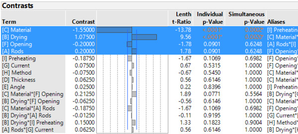
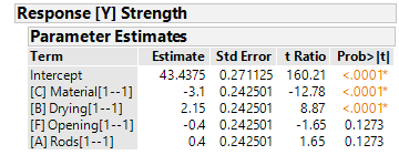
In the results of the (OLS) regression analysis, the influence of [C] and [B] on the tensile strength is confirmed. Even if [F] and [A] do not show a significant influence, one could still imagine to investigate these factors in more detail. As always, application knowledge must be decisive for model building.

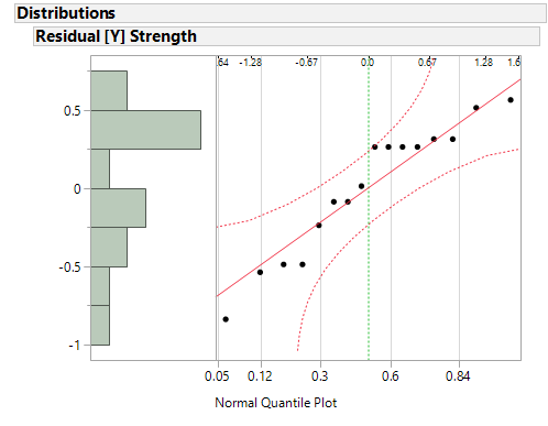
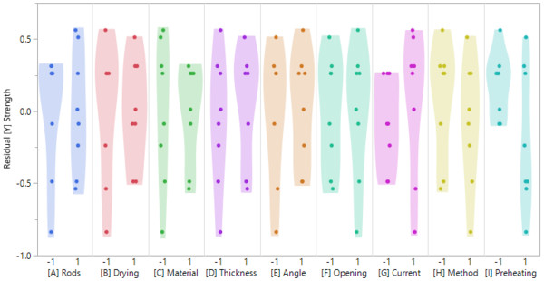
The normal quantile plot does not indicate a violation of the normal distribution assumption. Looking at the scatterplots of the individual factors versus the residuals, we see that the assumption of constant variances is not fulfilled everywhere. For the factors [B], [C], [G] and [I] the variance of the residuals seems to be different in the different factor levels. 

Apart from the fact that this violates one of our assumptions of the regression and thus the resulting p-values are no longer reliable, we already learn something about our process here: The mentioned factors seem to have an influence on the reproducibility of our results. If we look at factor [I], we see that the process seems to be quite robust for the low setting (-1). However, if one chooses the high setting (+1) one sees a high scatter in the data. This indicates a low reproducibility of the results.

Solution approaches 

There are a number of common recommendations for dealing with heteroscedasticity in the residuals: 

• Variable transformation: A Box-Cox-Power-Transformation can be helpful to find a suitable transformation of the target variable. Often the root or logarithm transformation proves to be variance stabilizing. 
• Use other models: Various Generalized Linear Regression (GLM) approaches allow non-constant variance as part of the model specification. 
• Heteroskedasticity Consistent Standard Errors: White standard errors take into account the presence of heteroskedasticity when calculating the standard errors of the regression and thus when calculating the p-values. 

All these methods have one thing in common: They try to solve the problem from a mathematical point of view. Either one tries to eliminate the heteroskedasticity (transformation) or to factor it out as part of the model specification.

If we use these methods, we typically do not get a deeper insight into the causes of heteroskedasticity. Especially when robustness is a central part of the optimization of a process, these are not suitable solutions. 

The loglinear Variance 

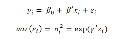
Model Another approach how to deal with the problem at hand are the Loglinear Variance Models (In the absence of a common name in science, I use the name from the JMP software for these models). The basic idea of these models is to model not only the mean of the target variables, but also the variance of the target variable at the same time. While simple linear regression uses only a mean equation

work Loglinear Variance Models with the following two equations:

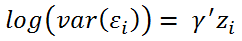
Obviously, the logarithm of the variance is described here by means of a linear predictor. The estimation of this model is, of course, somewhat more complex. Instead of the simple least squares method, a REML approach is used here. The procedure is described in detail by [G. Smyth 2002]. 

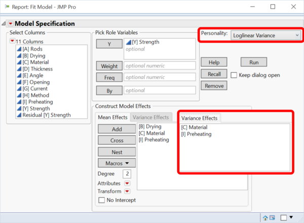
Example in JMP 

Before looking at the results of the model and their interpretation, it is important to realize that it is more laborious to estimate variances than means. Thus, estimating loglinear variance models requires more data than using simple regression models. In the present case, this means that we are not able to estimate a complete model. That is, a model in which all factors [A] to [I] are used to describe the mean and variance. 

So for this example, we stick to the model proposed by [Smyth 2002]: 

• The mean value is described by: [B], [C] and [I] 
• The variance is described by: [C] and [I] 

In JMP, the Loglinear Variance Models are found in the Fit Model platform.  

The p-values in the section "Mean Model for [Y] Strength" show us that [B] and [C] have a statistically significant effect on the tensile strength. Factor [I] is close to being statistically significant at the 5% significance level.  

In the section "Variance Model for [Y] Strength" we learn that the variance of the residuals (=reproducibility of the process) depends significantly on the factors [C] and [I].

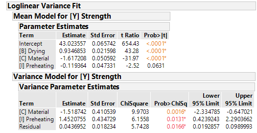
I.e. depending on which levels of [C] and [I] one works with, the process is more or less stable. Especially the influence of [I] - on mean and variance - is interesting, because the factor was completely left out in the simple regressio

For optimization we can work with the analysis diagram in JMP: The maximum tensile strength is achieved with high settings of [B] and low settings of [C]. The influence of [I] on the mean value is rather marginal. At the same time, [C] has a negative influence on the variance of the process. I.e. for maximizing the tensile strength we would like to have the lowest possible value of [C]. However, for the best possible reproducibility, [C] should be at a high level. It is easier with the factor [I]. The influence on the mean value is small. However, low settings of [I] lead to significantly lower variance and are therefore preferable. 

Conclusions 

1.  Loglinear models allow to model mean and variance at the same time. This opens up completely new possibilities, especially for the evaluation of D  
2. One problem, however, is that classical DoEs are only designed to estimate a pure mean model. I.e. many DoEs will not provide enough experiments to estimate a clean variance model at the same time. 
3. Point 2 also has an impact on model building, which in general has not yet been really explored. When it comes to modeling, however, purely statistical approaches can of course never be the solution. Application knowledge will always be needed here

Literature and useful sources 

1. M. Aitkin: Modelling Variance Heterogeneity in Normal Regression using GLIM (Journal of Royal Statistical Society. Series C (Applied Statistics), 1987) 
2. H. Goldstein: Heteroscedasticity and Complex Variation (Encyclopedia of Statistics in Behavioral Science) 
3. A.C. Harvey: Estimating Regression Models with Multiplicative Heteroiscedasticity (Econometrica, 1976) 
4. G. Smyth: An Efficient Algorithm for REML in Heteroscedastic Regression (Journal of Computational and Graphical Statistics, 2002) JMP 12 Online Documentation